j-invariant
In mathematics, Klein's j-invariant, regarded as a function of a complex variable τ, is a modular function defined on the upper half-plane of complex numbers.
We have
The modular discriminant  is defined as
The numerator and denominator above are in terms of the modular invariants  and
and  of the Weierstrass elliptic functions

and the modular discriminant.
These have the properties that


and possess the analytic properties making them modular forms. Δ is a modular form of weight twelve by the above, and one of weight four, so that its third power is also of weight twelve. The quotient is therefore a modular function of weight zero; this means j has the absolutely invariant property that

Contents |
Expressions in terms of theta functions
![g_2(\tau) = \tfrac12 \left[\vartheta(0;\tau)^8%2B\vartheta_{01}(0;\tau)^8%2B\vartheta_{10}(0;\tau)^8\right]](/2012-wikipedia_en_all_nopic_01_2012/I/9ff32cc6a0bae4be32d9083e4ee4efce.png)
![\Delta(\tau) = \tfrac12 \left[\vartheta(0;\tau) \vartheta_{01}(0;\tau) \vartheta_{10}(0;\tau)\right]^8.](/2012-wikipedia_en_all_nopic_01_2012/I/4821472d432fc03b335de1213abdc9aa.png)
We can express it in terms of Jacobi's theta functions, in which form it can very rapidly be computed.
![j(\tau) = 32 {[\vartheta(0;\tau)^8%2B\vartheta_{01}(0;\tau)^8%2B\vartheta_{10}(0;\tau)^8]^3 \over [\vartheta(0;\tau) \vartheta_{01}(0;\tau) \vartheta_{10}(0;\tau)]^8}.](/2012-wikipedia_en_all_nopic_01_2012/I/20d2ca04de49c661e1ff9be57c28be58.png)
The fundamental region
The two transformations  and
and  together generate a group called the modular group, which we may identify with the projective special linear group
  . By a suitable choice of transformation belonging to this group,
  , with ad − bc = 1, we may reduce τ to a value giving the same value for j, and lying in the fundamental region for j, which consists of values for τ satisfying the conditions

The function j(τ) takes on every value in the complex numbers  exactly once in this region. In other words, for every
  , there is a τ in the fundamental region such that c=j(τ). Thus, j has the property of mapping the fundamental region to the entire complex plane, and vice-versa.
As a Riemann surface, the fundamental region has genus 0, and every (level one) modular function is a rational function in j; and, conversely, every rational function in j is a modular function. In other words the field of modular functions is  .
.
The values of j are in a one-to-one relationship with values of τ lying in the fundamental region, and each value for j corresponds to the field of elliptic functions with periods 1 and τ, for the corresponding value of τ; this means that j is in a one-to-one relationship with isomorphism classes of elliptic curves over the complex numbers.
Class field theory and j
The j-invariant has many remarkable properties. One of these is that if τ is any element of an imaginary quadratic field with positive imaginary part (so that j is defined) then  is an algebraic integer. The field extension
![\mathbb{Q}[j(\tau),\tau]/\mathbb{Q}(\tau)](/2012-wikipedia_en_all_nopic_01_2012/I/f03bbbe8bccaccbc310518259ead9ff9.png)
is abelian, meaning with abelian Galois group. We have a lattice in the complex plane defined by 1 and τ, and it is easy to see that all of the elements of the field  which send lattice points to other lattice points under multiplication form a ring with units, called an order. The other lattices with generators 1 and τ' associated in like manner to the same order define the algebraic conjugates
  of over . The unique maximal order under inclusion of is the ring of algebraic integers of , and values of τ having it as its associated order lead to unramified extensions of . These classical results are the starting point for the theory of complex multiplication.
Transcendence properties
In 1937 Theodor Schneider proved the aforementioned result that if  is a quadratic irrational number in the upper half plane then j() is an algebraic integer. In addition he proved that if is an algebraic number but not imaginary quadratic then j() is transcendental.
The j function has numerous other transcendental properties. Kurt Mahler conjectured a particular transcendence result that is often referred to as Mahler's conjecture, though it was proved as a corollary of results by Yu. V. Nesternko and Patrice Phillipon in the 1990s. Mahler's conjecture was that the if was in the upper half plane then exp(2πi) and j() were never both simultaneously algebraic. Stronger results are now known, for example if exp(2πi) is algebraic then the following three numbers are algebraically independent, and thus transcendental:
The q-expansion and moonshine
Several remarkable properties of j have to do with its q-expansion (Fourier series expansion, written as a Laurent series in terms of  ), which begins:

Note that j has a simple pole at the cusp, so its q-expansion has no terms below  .
.
All the Fourier coefficients are integers, which results in several almost integers, notably Ramanujan's constant : .
.
Moonshine
More remarkably, the Fourier coefficients for the positive exponents of q are the dimensions of the graded part of an infinite-dimensional graded algebra representation of the monster group called the moonshine module – specifically, the coefficient of  is the dimension of grade-n part of the moonshine module, the first example being the Griess algebra, which has dimension 196,884, corresponding to the term
  This startling observation was the starting point for moonshine theory.
The study of the Moonshine conjecture led J.H. Conway and Simon P. Norton to look at the genus-zero modular functions. If they are normalized to have the form

then Thompson showed that there are only a finite number of such functions (of some finite level), and Cummins later showed that there are exactly 6486 of them, 616 of which have integral coefficients..
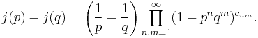
A remarkable property of the q-series for j is the product formula; if p and q are small enough we have
Algebraic definition
So far we have been considering j as a function of a complex variable. However, as an invariant for isomorphism classes of elliptic curves, it can be defined purely algebraically. Let

be a plane elliptic curve over any field. Then we may define


and

the latter expression is the discriminant of the curve.
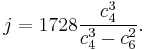
The j-invariant for the elliptic curve may now be defined as

In the case that the field over which the curve is defined has characteristic different from 2 or 3, this definition can also be written as
Inverse and special values
The inverse of the j-invariant can be expressed in terms of the hypergeometric function  (see main article Picard–Fuchs equation). The inversion of the j-invariant was reported by Semjon Adlaj (CCRAS, Moscow, Russia) on May 30, 2011 prior to a talk given at the 14-TH WORKSHOP ON COMPUTER ALGEBRA (Dubna, Russia). The inversion is highly relevant to applications via enabling high precision calculations of elliptic functions periods even as their ratios become unbounded. A related result is the expressability via quadratic radicals of the values of j at the points of the imaginary axis whose magnitudes are powers of 2 (thus permitting compass and straightedge constructions). The latter result is hardly evident since the modular equation of level 2 is cubic. For example, the value of j at
  simplifies(!) to:
![\begin{align}
j(4 i) & = \frac{1}{108} \left( \frac{33}{8} \left( \left( \sqrt{- 3} %2B 1 \ \right) \sqrt[3]{21 \sqrt{- 3 / 8} - 1} - \frac{11 \left( \sqrt{- 3} - 1 \right)}{\sqrt[3]{42 \sqrt{- 6} - 8}} \right) %2B 1 \right) \times \\
& {} \quad \times \left( \frac{256}{16 - 33 \left( 11 \left( \sqrt{- 3} - 1 \ \right) / \sqrt[3]{21 \sqrt{- 3 / 8} - 1} - \left( \sqrt{- 3} %2B 1 \ \right) \sqrt[3]{42 \sqrt{- 6} - 8} \right)} - 1 \right)^3.
\end{align}](/2012-wikipedia_en_all_nopic_01_2012/I/f770135b7a843bd2ae9b4a02ed8a0cd2.png)
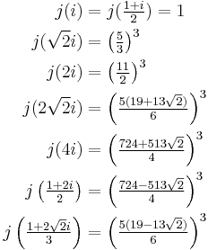
The j-invariant vanishes at the "corner" of the fundamental domain at  . Here are seven more special values (only the first four of which are well known):
References
- Apostol, Tom M. (1976), Modular functions and Dirichlet Series in Number Theory, Graduate Texts in Mathematics, 41, New York: Springer-Verlag, MR0422157. Provides a very readable introduction and various interesting identities.
- Apostol, Tom M. (1990), Modular functions and Dirichlet Series in Number Theory (2nd ed.), ISBN 0-387-97127-0, MR1027834
- Berndt, Bruce C.; Chan, Heng Huat (1999), "Ramanujan and the modular j-invariant", Canadian Mathematical Bulletin 42 (4): 427–440, doi:10.4153/CMB-1999-050-1, MR1727340, http://www.journals.cms.math.ca/cgi-bin/vault/public/view/berndt7376/body/PDF/berndt7376.pdf. Provides a variety of interesting algebraic identities, including the inverse as a hypergeometric series.
- Conway, John Horton; Norton, Simon (1979), "Monstrous moonshine", Bulletin of the London Mathematical Society 11 (3): 308–339, doi:10.1112/blms/11.3.308, MR0554399. Includes a list of the 175 genus-zero modular functions.
- Petersson, Hans (1932), "Über die Entwicklungskoeffizienten der automorphen Formen", Acta Mathematica 58 (1): 169–215, doi:10.1007/BF02547776, MR1555346.
- Rademacher, Hans (1938), "The Fourier coefficients of the modular invariant j(τ)", American Journal of Mathematics (The Johns Hopkins University Press) 60 (2): 501–512, doi:10.2307/2371313, JSTOR 2371313, MR1507331.
- Rankin, Robert A. (1977), Modular forms and functions, Cambridge: Cambridge University Press, ISBN 0-521-21212-X, MR0498390. Provides a short review in the context of modular forms.
- Schneider, Theodor (1937), "Arithmetische Untersuchungen elliptischer Integrale", Math. Annalen 113: 1–13, doi:10.1007/BF01571618, MR1513075.